Specifying the Model - Full Model
Now let’s specify and test the full model, with multiple inputs and multiple outputs.
Model Overview
Restating what I put at the top of the overview notebook
\[ y_{t+1} \sim N(\beta_t X_t, \Sigma_y) \\ \beta_d \sim MN(0, \Sigma_{N,d}, \Sigma_{\beta}) \\ \Sigma(N, d)_{i,j} = \alpha_d^2exp\left (-\frac{1}{2\rho_d^2}(i-j)^2 \right ) + \delta_{i,j}\\ \rho_d \sim \gamma^{-1}(5,5) \\ \begin{matrix}\alpha_d \sim N(0, 1) & \alpha > 0 \end{matrix} \]
\[ \delta_{i,j} \{\begin{matrix} \sim N(0,1) & i \equiv j\\ 0 & i \neq j \end{matrix} \]
\[ \Sigma_\beta = \Omega_\beta'\tau\Omega_\beta \\ \Omega_\beta \sim LJKCorr(3) \\ \tau \sim cauchy(0, 1), \tau > 0 \]
\[ \Sigma_y = \Omega_y'\sigma\Omega_y \\ \Omega_y \sim LJKCorr(4) \\ \sigma_a \sim cauchy(0, 1), \sigma_a > 0 \]
As I mentioned in the last notebook, I think I’m not going to model \(\Sigma_y\), but instead specify the covariance matrix based on the exponentially-weighted historical values.
The trickiest bit here is going to be specifying a matrix-variate distribution for \(\beta\). Stan does not have one built in1, so I’m going to have to write a set of functions to use a multivariate normal distribution instead. Basically, matrix-variate should be equivalent to a multivariate distribution in which the additional axis has been stacked vertically for \(\mu\), and the \(\Sigma\) is the Kronecker product of \(\Sigma_{N}\) and \(\Sigma_\beta\). This should be ringing bells for anybody familiar with Zellner’s Seemingly Unrelated Regressions, too. Unfortunately, Stan doesn’t implement the Kronecker product, either. If you go through the Stan discussion board and the old mailing list, the advice seems to be, “try hard not to need the full matrix created by the Kronecker product”. But I lack the math to implement matrix-normal efficiently in Stan. Mike Shvartsman gives the basis for an efficient, cholesky-based implementation of the likelihood for a matrix-normal, but this hasn’t been incorporated into Stan-dev. I defer to the experts; there have been discussions on the subject for several years, and as Gaussian Processes seem to be getting trendier these days, something may come of them soon. If my implementation winds up being too slow, which is pretty likely, we may need to switch to TensorFlow or some other machine learning library after validating in Stan’s generative version. Or, it may be that the generative model is too slow, but just calling optimize on it is adequate.
Instead of writing the model directly with a matrix-variate normal distribution, I’m going to follow Rob Trangucci’s demonstration of hiearchical GPs from this year’s Stan conference.
knitr::opts_chunk$set(warning = FALSE, message = FALSE)
library(tidyverse)
library(rstan) #2.17 hasn't been released yet for rstan, but we'll be using cmdstan 2.17.
rstan_options(auto_write = TRUE)
options(mc.cores = parallel::detectCores())
As before, this model can be found in the stan directory.
cat(read_file("../stan/gp.stan"))// Full gp model, in which beta is matrix-variate
// wound up implementing the beta variance via
// hierarchy, as in Trangucci's work.
data {
int<lower=1> N; // # of dts
int<lower=1> A; // # of endos
int<lower=1> B; // # of betas
matrix[N,A] y;
matrix[B,A] x[N]; // Exog
cov_matrix[A] y_cov[N]; //contemporaneous covariance of ys
}
transformed data {
real t[N];
matrix[A,A] L_y_cov[N];
real delta = 1e-9;
vector[B] beta_mu_mu = rep_vector(0, B);
for(n in 1:N) {
t[n] = n;
L_y_cov[n] = cholesky_decompose(y_cov[n]);
}
}
parameters {
matrix[N,B] beta;
real<lower=0> alpha[B];
vector<lower=0>[B] sigma;
real<lower=0> length_scale[B];
cholesky_factor_corr[B] L_omega; //eta correlation
matrix[N,B] beta_mu; //Instead of 0s, I'm going to
//put the beta-wise covariance on this term to avoid
//having a massive kronecker product matrix.
}
model {
matrix[N,N] cov[B];
matrix[B,B] L_Sigma_b;
to_vector(alpha) ~ normal(0.5, 1);
sigma ~ cauchy(0, 1);
L_omega ~ lkj_corr_cholesky(4);
L_Sigma_b = diag_pre_multiply(sigma, L_omega);
for(b in 1:B)
cov[b] = cov_exp_quad(t, alpha[b], length_scale[b]);
for(n in 1:N) {
beta_mu[n] ~ multi_normal_cholesky(beta_mu_mu, L_Sigma_b);
for(b in 1:B)
cov[b, n, n] = cov[b, n, n] + delta;
}
for(b in 1:B)
beta[,b] ~ multi_normal_cholesky(beta_mu[,b], cholesky_decompose(cov[b]));
for(n in 1:N)
y[n] ~ multi_normal_cholesky(beta[n] * x[n], L_y_cov[n]);
}This is substantially different from the code for single asset, because I wanted to avoid making mistakes in vectorizing over two different dimensions (both exogs and endos). This format is much more readable. Also note I’m specifying a fixed endogenous covariance, rather than estimating. This is to reduce parameters. You could plug GARCH in here directly, or fit a GARCH model separately and provide that. I would be inclined to stick in plain EWMA (exponentially weighted moving average) endogenous covariance, as I’ve not seen much improvement when using GARCH in these macro FX models in the past. For now, let’s do our fake data simulation and parameter recovery test with the constant endogenous covariance matrix.
Generating Fake Data
Betas and beta correlation will be generated using Stan functions, like last time.
sim_model <- stan_model(model_name="sim_full", file="../stan/gp_sim.stan")rstan::expose_stan_functions(sim_model)
set.seed(8675309) #Let's keep the randomness consistent
fake_data = list(N=100, B=3, A=2, alpha=c(0.1, 0.25, 0.5),
length_scale=c(0.8, 0.9, 1.0),
sigma=c(0.025, 0.05, 0.075))
fake_data <- within(fake_data, {
x <- array(rnorm(N*B*A, sd=0.1), dim=c(N,B,A))
L_omega <- rho_rng(B, 4)
beta <- eta_rng(N, B, alpha, length_scale, sigma, L_omega)
y_cov <- aperm(array(diag(c(0.01,0.05)) %*% tcrossprod(rho_rng(A, 3)) %*% diag(c(0.01,0.05)),
dim=c(A,A,N)), c(3,1,2))
})fake_data$beta %>% as_tibble() %>% mutate(t=seq.int(100)) %>%
gather(beta,value, -t) %>% ggplot(aes(x=t,y=value,col=beta)) +
geom_line() + ggtitle("Fake betas over time")
with(fake_data,x[,,1]*beta) %>% as_tibble() %>% mutate(t=seq.int(100)) %>%
  gather(beta,value, -t) %>% ggplot(aes(x=t,y=value,col=beta)) +
  geom_line() + ggtitle("Fake XBs over time (asset 1)")
Simulate endos
sim_samples <- sampling(sim_model, fake_data, chains=2, algorithm="Fixed_param") #algorithm='Fixed_param' is a new one for me.Now we have 2000 possible series based on those parameters. Let’s see how different they are. We’re going to wind up using the median to test recovering parameters.
library(reshape2)
sim_y <- extract(sim_samples)$y
sim_y %>% melt(varnames=c("iteration", "time", "asset")) %>%
  filter(iteration %in% sample.int(2000,100)) %>%
  ggplot(aes(x=time,y=value, group=iteration)) + facet_wrap(~asset, ncol=1) +
  geom_line(alpha=0.05) + ggtitle("Y sims")
Once again, not much variation compared to what we’ll see in the real data, as these endos really are driven solely by \(X\beta\).
Recover Known Parameters
Same drill as before.
gp_model <- stan_model(file="../stan/gp.stan", model_name='gp')
fake_data <- within(fake_data, {y<-apply(sim_y,c(2,3),median)})
gp_fit <- sampling(gp_model, fake_data[c("N","A","B","y","x","y_cov","sim")], chains=3, cores=3) #This one will take a while, and I only have 4 physical cores on this machine.
That took 5 hours on my laptop. We had 3 exogs and 2 endos. The full model has 5 exogs and 11 assets. However, it only took 1.2 hours on the VM Syracuse has provided me! So I’ve got that going for me.
Now, did it work?
stopifnot(require(bayesplot))
mcmc_trace(as.array(gp_fit), pars=c("alpha[1]", "length_scale[2]", "L_omega[2,1]",
                                        "L_omega[3,2]", "L_omega[3,1]",
                                            "sigma[2]"))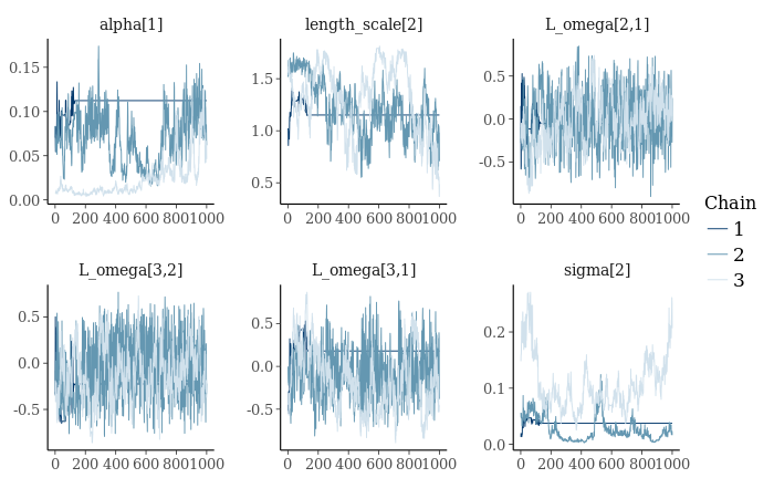
That’s not good. Looks like we have a stuck chain. Also, poor mixing on sigma and alpha. I might try again with a different random seed. First let’s take a better look at parameter recovery.
index_it <- function(x,i) {paste0(x,"[",i,"]")}
gp_fit_array <- as.array(gp_fit)
mcmc_recover_intervals(gp_fit_array[,,grep("(alpha|length_scale|sigma)", dimnames(gp_fit_array)$parameters)],
                             true=with(fake_data,c(alpha,sigma,length_scale))) + coord_flip()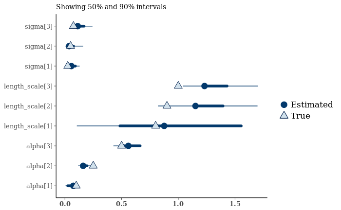
Not too bad, but the stuck chain is pretty visible. Let’s look at histograms.
mcmc_recover_hist(gp_fit_array[,,grep("(alpha|length_scale|sigma)", dimnames(gp_fit_array)$parameters)],
                             true=with(fake_data,c(alpha,sigma,length_scale)))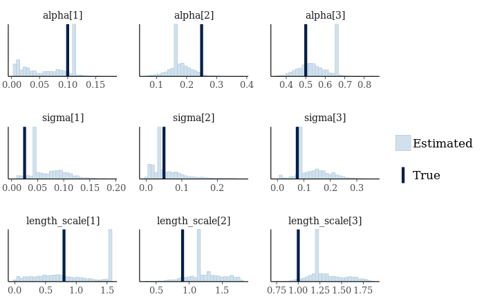
Ok, time to try fitting a second time. I’m going to change the random seed, throw another chain on there, and add 1000 iterations.
gp_fit <- sampling(gp_model, fake_data[c("N","A","B","y","x","y_cov","sim")],
                   chains=4, cores=4, iter=3000, seed=9178675309)
2.2 hours. Not bad. Looks like my seed was too big though. Shouldn’t give Jenny an area code.
stopifnot(require(bayesplot))
gp_fit_array <- as.array(gp_fit)
mcmc_recover_hist(gp_fit_array[,,grep("(alpha|length_scale|sigma)", dimnames(gp_fit_array)$parameters)],
                             true=with(fake_data,c(alpha,sigma,length_scale)))
That’s better. Well-mixed?
mcmc_trace(as.array(gp_fit), pars=c("alpha[1]", "length_scale[2]", "L_omega[2,1]",
                                        "L_omega[3,2]", "L_omega[3,1]",
                                            "sigma[2]"))
Ug. Might need more like 5000 to get everything mixed properly. Let’s see how good the optimizer is. This will do MAP instead of generative modeling.
gp_optim <- optimizing(gp_model, fake_data[c("N","A","B","y","x","y_cov","sim")],
                  iter=5000, algorithm="BFGS")
## Initial log joint probability = -5.47208e+10
## Exception: cov_exp_quad: l is 0, but must be > 0! (in 'model3d48583c47d3_gp' at line 42)
##
## Exception: cov_exp_quad: l is 0, but must be > 0! (in 'model3d48583c47d3_gp' at line 42)
##
## Exception: cov_exp_quad: l is 0, but must be > 0! (in 'model3d48583c47d3_gp' at line 42)
##
## Exception: cov_exp_quad: l is 0, but must be > 0! (in 'model3d48583c47d3_gp' at line 42)
##
## Exception: cov_exp_quad: l is 0, but must be > 0! (in 'model3d48583c47d3_gp' at line 42)
##
## Exception: cov_exp_quad: l is 0, but must be > 0! (in 'model3d48583c47d3_gp' at line 42)
##
## Exception: cov_exp_quad: l is 0, but must be > 0! (in 'model3d48583c47d3_gp' at line 42)
##
## Exception: cov_exp_quad: l is 0, but must be > 0! (in 'model3d48583c47d3_gp' at line 42)
##
## Exception: cov_exp_quad: l is 0, but must be > 0! (in 'model3d48583c47d3_gp' at line 42)
##
## Exception: cov_exp_quad: l is 0, but must be > 0! (in 'model3d48583c47d3_gp' at line 42)
##
## Exception: cov_exp_quad: l is 0, but must be > 0! (in 'model3d48583c47d3_gp' at line 42)
##
## Exception: cov_exp_quad: l is 0, but must be > 0! (in 'model3d48583c47d3_gp' at line 42)
##
## Exception: cov_exp_quad: l is 0, but must be > 0! (in 'model3d48583c47d3_gp' at line 42)
##
## Exception: cov_exp_quad: l is 0, but must be > 0! (in 'model3d48583c47d3_gp' at line 42)
##
## Exception: cov_exp_quad: l is 0, but must be > 0! (in 'model3d48583c47d3_gp' at line 42)
##
## Exception: cov_exp_quad: l is 0, but must be > 0! (in 'model3d48583c47d3_gp' at line 42)
##
## Error evaluating model log probability: Non-finite gradient.
## Error evaluating model log probability: Non-finite gradient.
##
## Error evaluating model log probability: Non-finite gradient.
## Error evaluating model log probability: Non-finite gradient.
##
## Optimization terminated with error:
## Line search failed to achieve a sufficient decrease, no more progress can be madedata.frame(par_hat=gp_optim$par[grep("(alpha|length_scale|sigma)", names(gp_optim$par))],
par=with(fake_data,c(alpha,sigma,length_scale)))## par_hat par
## alpha[1] 8.589032e-15 0.100
## alpha[2] 5.945854e-19 0.250
## alpha[3] 1.458044e-13 0.500
## sigma[1] 4.294421e-05 0.025
## sigma[2] 8.796084e-01 0.050
## sigma[3] 3.988476e-01 0.075
## length_scale[1] 2.420502e-01 0.800
## length_scale[2] 3.366310e-22 0.900
## length_scale[3] 2.190046e-01 1.000Pretty far off. I’ve tried tweaking a few parameters around this, but it looks like optimization just may not work for this model. Lord knows the posterior is going to be multimodal on this.
This means the backtest is going to require a lot of hardware.
Next up, real data.
Next: Forecasting
Actually, there is one in the Stan code, but it’s not exposed, presumably with good reason.↩